SUPPORT VECTOR MACHINES
1. SVM with various kernels
The SVM command is in package called e1071.
> install.packages("e1071");
> library(e1071)
Let’s use support vector machines to classify cars into Economy and Consuming classes.
> ECO = ifelse( mpg > 22.75, "Economy", "Consuming" )
> Color = ifelse( mpg > 22.75, "green", "red" )
> plot( weight, horsepower, lwd=3, col=Color )
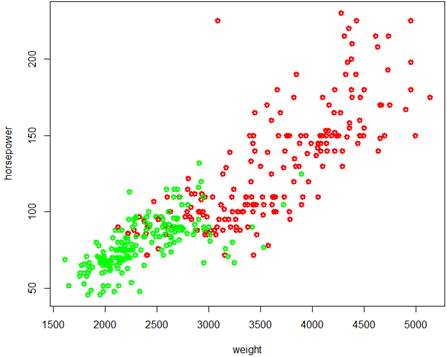
The two classes cannot be separated by a hyperplane, but the SVM method is surely applicable.
> S = svm( ECO ~ weight + horsepower, data=Auto, kernel = "linear" )
Error in svm.default(x, y, scale = scale, ..., na.action = na.action) :
Need numeric dependent variable for regression.
Error? There are other, unused variables in dataset Auto that prevent R from doing this SVM analysis. We’ll create a reduced dataset.
> d = data.frame(ECO, weight, horsepower)
> S = svm( ECO ~ weight + horsepower, data=d, kernel="linear" )
> summary(S)
Parameters:
SVM-Type: C-classification
SVM-Kernel: linear
cost: 1
gamma: 0.5
Number of Support Vectors: 120
( 60 60 )
So, there are 120 points violating the separating hyperplane or the margin, 60 in each class.
> plot(S, data=Auto)
Error in plot.svm(S, data = Auto) : missing formula.
Same story. We need to use a reduced dataset that contains only the needed variables.
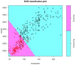
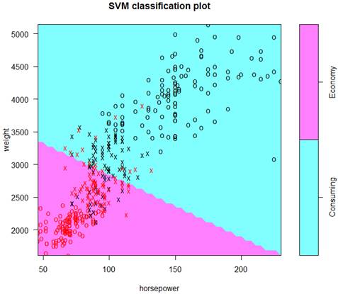
> plot(S, data=d)
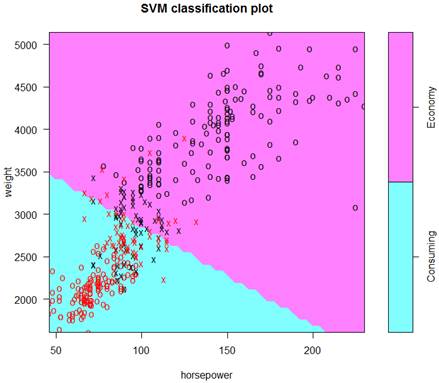
This is the final classification with a linear kernel and therefore, a linear boundary. Support vectors are marked as “x”, other points as “o”.
We can look at other types of kernels and boundaries – polynomial, radial, and sigmoid.
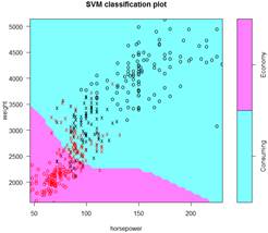
> S = svm( ECO ~ weight + horsepower, data=d, kernel="polynomial" )
> summary(S); plot(S,d)
Number of Support Vectors: 176
> S = svm( ECO ~ weight + horsepower, data=d, kernel="radial" )
> summary(S); plot(S,d)
Number of Support Vectors: 121
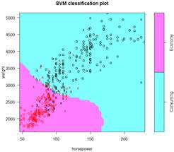
> S = svm( ECO ~ weight + horsepower, data=d, kernel="sigmoid" )
> summary(S); plot(S,d)
Number of Support Vectors: 74
Adding more variables should give a better fit – to the training data.
> S = svm( factor(ECO) ~ weight + horsepower + displacement + cylinders, data=Auto, kernel="linear" )
> summary(S)
Number of Support Vectors: 99
We can identify the support vectors:
> S$index
[1] 16 17 18 25 33 45 46 48 60 61 71 76 77 78 80 100 107 108 109
[20] 110 111 112 113 119 120 123 153 154 162 173 178 199 206 208 209 210 240 241
[39] 242 253 258 262 269 273 274 275 280 281 384 24 31 49 84 101 114 122 131
[58] 149 170 177 179 192 205 218 233 266 270 271 296 297 298 299 305 306 313 314
[77] 318 322 326 327 331 337 338 353 355 356 357 358 360 363 365 368 369 375 381
[96] 382 383 385 387
> Auto[S$index,]
mpg cylinders displacement horsepower weight acceleration year origin
16 22.0 6 198 95 2833 15.5 70 1
17 18.0 6 199 97 2774 15.5 70 1
18 21.0 6 200 85 2587 16.0 70 1
25 21.0 6 199 90 2648 15.0 70 1
< truncated >
2. Tuning and cross-validation
The “cost” option specifies the cost of violating the margin. We can try costs 0.001, 0.01, 0.1, 1, 10, 100, 1000:
> Stuned = tune( svm, ECO ~ weight + horsepower, data=d, kernel="linear", ranges=list(cost=10^seq(-3,3)) )
> summary(Stuned)
- sampling method: 10-fold cross validation
- best parameters:
cost
0.1
- best performance: 0.1173718
- Detailed performance results:
cost error dispersion
1 1e-03 0.2478205 0.10663023
2 1e-02 0.1432051 0.05485355
3 1e-01 0.1173718 0.04208311 # This cost yielded the lowest cross-validation error of classification.
4 1e+00 0.1326282 0.04461101
5 1e+01 0.1351923 0.04819639
6 1e+02 0.1351923 0.04819639
7 1e+03 0.1351923 0.04819639
We can also find the optimal kernel.
> Stuned = tune( svm, ECO ~ weight + horsepower, data=d, ranges=list(cost=10^seq(-3,3), kernel=c("linear","polynomial","radial","sigmoid")) )
> summary(Stuned)
Parameter tuning of ‘svm’:
- sampling method: 10-fold cross validation
- best parameters:
cost kernel
0.1 sigmoid
- best performance: 0.1046154
- Detailed performance results:
cost kernel error dispersion
1 1e-03 linear 0.2164744 0.10501351
2 1e-02 linear 0.1326282 0.05074006
3 1e-01 linear 0.1096154 0.04330918
4 1e+00 linear 0.1172436 0.03813782
5 1e+01 linear 0.1223718 0.04775672
6 1e+02 linear 0.1223718 0.04775672
7 1e+03 linear 0.1223718 0.04775672
8 1e-03 polynomial 0.3720513 0.08274072
9 1e-02 polynomial 0.2601282 0.06438244
10 1e-01 polynomial 0.1987821 0.07443903
11 1e+00 polynomial 0.1784615 0.05328633
12 1e+01 polynomial 0.1580769 0.04909157
13 1e+02 polynomial 0.1555128 0.04999836
14 1e+03 polynomial 0.1504487 0.04722372
15 1e-03 radial 0.5816026 0.05687780
16 1e-02 radial 0.1301282 0.05190241
17 1e-01 radial 0.1198077 0.05104329
18 1e+00 radial 0.1223718 0.04118608
19 1e+01 radial 0.1096795 0.04835338
20 1e+02 radial 0.1198718 0.04184981
21 1e+03 radial 0.1146795 0.04354410
22 1e-03 sigmoid 0.5816026 0.05687780
23 1e-02 sigmoid 0.1530769 0.04517581
24 1e-01 sigmoid 0.1046154 0.03711533 # The best kernel and cost.
25 1e+00 sigmoid 0.1173718 0.04715638
26 1e+01 sigmoid 0.1530769 0.06159616
27 1e+02 sigmoid 0.1582051 0.06489946
28 1e+03 sigmoid 0.1582051 0.06489946
> Soptimal = svm( ECO ~ weight + horsepower, data=d, cost=0.1, kernel="sigmoid" )
> summary(Soptimal); plot(Soptimal,data=d)
Parameters:
SVM-Type: C-classification
SVM-Kernel: sigmoid
cost: 0.1
gamma: 0.5
Number of Support Vectors: 164 # We know that more support vectors imply a lower variance
( 82 82 )
Number of Classes: 2
Levels: Consuming Economy
Let’s use the validation set method to estimate the classification rate of this optimal SVM.
> n = length(mpg); Z = sample(n,n/2)
> Strain = svm( ECO ~ weight + horsepower, data=d[Z,], cost=0.1, kernel="sigmoid" )
> Yhat = predict( Strain, data=d[-Z,] )
> table( Yhat, ECO[Z] )
Yhat Consuming Economy
Consuming 82 9
Economy 17 88
> table( Yhat, ECO[Z] )
> mean( Yhat==ECO[Z] )
[1] 0.8673469
3. More than two classes
Let’s create more categories of ECO. The same tool svm( ) can handle multiple classes.
> summary(mpg)
Min. 1st Qu. Median Mean 3rd Qu. Max.
9.00 17.00 22.75 23.45 29.00 46.60
> ECO4 = rep("Economy",n)
> ECO4[mpg < 29] = "Good"
> ECO4[mpg < 22.75] = "OK"
> ECO4[mpg < 17] = "Consuming"
> table(ECO4)
ECO4
Consuming Economy Good OK
92 103 93 104
> S4 = svm( ECO4 ~ weight + horsepower, data=d, cost=0.1, kernel="sigmoid" )
Error in svm.default(x, y, scale = scale, ..., na.action = na.action) :
Need numeric dependent variable for regression.
R was trying to do regression SVM but realized that ECO4 is not numerical. We can direct R to do classification by replacing ECO4 with factor(ECO4).
> S4 = svm( factor(ECO4) ~ weight + horsepower, data=d, cost=0.1, kernel="sigmoid" )
> plot(S4, data=d)
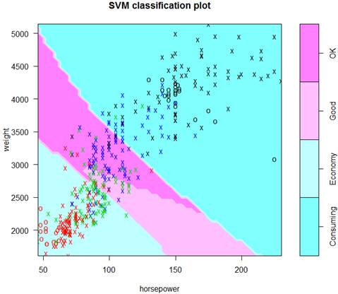
> Yhat = predict( S4, data.frame(Auto) )
> table( Yhat, ECO4 )
ECO4
Yhat Consuming Economy Good OK
Consuming 88 0 2 33
Economy 0 96 58 15
Good 0 2 9 5
OK 4 5 24 51
> mean( Yhat == ECO4 )
[1] 0.622449
It’s more difficult to predict finer classes correctly